Sines and cosines for fun and profit
Hi everybody! This article will be a voyage through some simple effects, with a very distinctive oldskool look, all of which are obtained by combining in various clever ways the two basic trigonometric functions, sine and cosine. What's interesting is that all of these effects don't require a very deep knowledge of math, and so can be a good source of satisfaction for newbies before they attack more complex things like 3D. In the end I will present two effects that do use some math and even a little 3D projection (rotozooming and wormholes), but don't worry as I will guide you through the couple of equations you need. The only knowledge that I require is that you know how to operate in graphics mode (plot a pixel, set a palette, load a bitmap from disk and draw it).
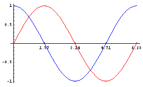
The first effects that I present are based on the following fundamental syllogism: we want to draw nice pictures, the sine and cosine functions have nice curves, i.e. we'll use sines and cosines -- without even knowing what they are about, at least at first. Here are the curves of the sine (red) and cosine (blue):
These effects have not been used in demos for years, but they can be a useful source of inspiration in little "for fun" productions like 256 byte or 4k intros.
Plasmas
Plasmas are a very simple effect. They are nothing more than patterns that evolve over time, creating colored blobs that emerge and disappear; they are not very interesting on their own, but they can be combined in a lot of interesting ways: for example you can draw two plasmas and plot them in alternate pixels, giving a nice interference figure; or you can use them as texture or bump maps; or again, you can draw each point in the plasma as a small sprite (e.g. 8x8) instead of plotting single pixels. Anyway, I guess that every coder wrote a plasma routine once in his life, so why shouldn't you?
How do we do a plasma? A first property we must know of sines and cosines is that when you sum many of them they combine in unpredictable ways: their curves have areas in which they change very slowly and areas in which their slope is much more steep. All this, however, happens without any solution of continuity.
We will shift over time all of the curves that we sum; some of them will also depend on the x coordinate and some others on the y. The equation will be therefore something like:
        32 (cos (a x + b t + c) +
            cos (d x + e t + f) +
            cos (g y + h t + i) +
            cos (j y + k t + l) + 4)
Each cosine goes from -1 to 1, so when you sum four of them the result goes from -4 to 4. The two adjustment factors, 4 and 32, make it go from 0 to 255 instead. This is good as we will operate in a 256-color palettized mode.
I'm using only cosines because sines are simply cosines with the argument shifted by PI/2, and traditionally plasmas are coded with cosines, but sines work as well if you prefer. Of course we will not afford to compute four cosines per pixel, because another property of the sine and cosine function is that it's quite expensive to compute them (Hugi 23 had two articles by Adok and me on this topic). But sines and cosines repeat continuously as their arguments change by 2PI, so we can make a table with a few values of the cosine with the argument ranging from 0 to 2PI, and reuse the values in this table.
We will make the size of the table a nice power of two, so that the modulus can be computed with a bitwise AND, and scale the values from 0 to 63 so that we only have to sum them: the new formula is, if the cosine table has 256 entries,
          cosTable [(a x + b t + c) & 255] +
          cosTable [(d x + e t + f) & 255] +
          cosTable [(g y + h t + i) & 255] +
          cosTable [(j y + k t + l) & 255]
Now we have to pick the values of the parameters. Well, we just try until the result satisfies us, starting from low integers and varying them until the result has a pleasing speed and look. I will give you a single hint: if two parameters have the same position in the equation (for example, both multiply a coordinate or both multiply t), don't make them equal, otherwise the curve will lose much of its unpredictability.
The pseudocode then looks like this:
     enter gfx mode and set the palette
     for i := 0 to 255 do
       cosTable[i] := 32 + 32 * cos (i * 2*PI/256)
     end;

     for each frame
       for each pixel
         plot (x,y) with a color given by the formula above
We can also economize on the multiplication by keeping track of the values of the cosines. The timeX variables track terms like b*t+c, while angleX track the arguments of the cosines (which, as you might already know, are angles):
     enter gfx mode and set the palette
     for i = 0 to 255
       cosTable[i] := 32 + 32 * cos (i * 2*PI/256)

     time1 := c
     time2 := f
     time3 := i
     time4 := l

     for each frame
       angle3 := time3
       angle4 := time4
       for y := 0 to maxy - 1 do
         angle1 := time1
         angle2 := time2
         for x := 0 to maxx - 1 do
           color := cosTable[angle1 & 255] + cosTable[angle2 & 255] +
                    cosTable[angle3 & 255] + cosTable[angle4 & 255];

           plot (x,y) with this color
           angle1 := angle1 + a
           angle2 := angle2 + d
         end;
         angle3 := angle3 + g
         angle4 := angle4 + j
       end;

       time1 := time1 + b
       time2 := time2 + e
       time3 := time3 + h
       time4 := time4 + k
     end;
That's it. You have a plasma. You can try other variations on this theme, for example:
            cos (cos (a x + b t + c) + d t + e) +
            cos (cos (f y + g t + h) + i t + j) +
                 cos (a x + b t + c) +
                 cos (f y + g t + h)
I will leave to you the task of optimizing it to remove the multiplications. Also, try to invent and code some creative combinations of plasmas, like the ones I outlined above.
Interference
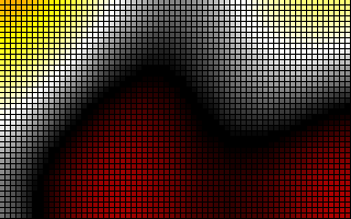
Interference is another basic effect which combines sines and cosines. Instead of computing many cosines and sum them together, you use each of them as a coordinate into a texture, and sum the pixel values of the textures:
Since the textures themselves will frequently be computed using formulas based on sines and cosines, it makes sense to remove the x and y terms from the cosines, and simply turn
256 cos (a x + b t + c)
into
(x + 256 cos (b t + c)) & 255
so that what the effect does is simply to shift the textures by a different amount on each frame.
Note that with this change you can do the lookup in the cosine table once per frame, instead of once per pixel. Actually this makes it possible to remove the table altogether and use floating point arithmetic, because you only have to compute a handful of cosines per frame.
The following pseudocode assumes that textures are 256x256. To make things more interesting, I will rotate the palette on each frame, which is easily done by summing the frame number to the color of the pixel.
        x1_angle = 0; x2_angle = 0; x3_angle = 0; x4_angle = 0
        y1_angle = 0; y2_angle = 0; y3_angle = 0; y4_angle = 0
        t := 0

        for each frame
          increment the XX_angle by a small number (up to 0.05)
          x1 := (cos (x1_angle) + 1) * 128
          y1 := (cos (y1_angle) + 1) * 128
          x2 := (cos (x2_angle) + 1) * 128
          y2 := (cos (y2_angle) + 1) * 128
          x3 := (cos (x3_angle) + 1) * 128
          y3 := (cos (y3_angle) + 1) * 128
          x4 := (cos (x4_angle) + 1) * 128
          y4 := (cos (y4_angle) + 1) * 128
          t := t + 1

          for y := 0 to maxy - 1 do
            for x := 0 to maxx - 1 do
              plot (x,y) with color
                texture1[(x1+x) & 255, (y1+y) & 255] +
                texture1[(x2+x) & 255, (y2+y) & 255] +
                texture2[(x3+x) & 255, (y3+y) & 255] +
                texture2[(x4+x) & 255, (y4+y) & 255] + t;
You can put whatever you like in this textures, for example a turbulence function (i.e. the altitude of a fractal landscape -- there are plenty of tutorials for this) or a pattern from your favorite drawing program, like 3D-Studio or the GIMP. But I will explain how to draw simple algorithmic textures with (of course) sines and cosines.
Here are the two textures that were used for the image above:
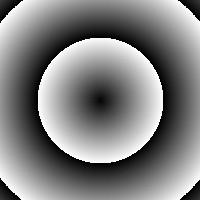
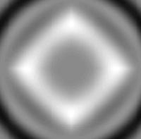
The left one is very simple. The function sqrt(x*x+y*y) will give the distance from the origin to a point (this is nothing more than Pythagoras' theorem...), and we want to give the same color to points with the same distance.
If you view the texture in a painting program and compute the distances of a few points (painting programs usually show the coordinates somewhere), you'll see that black points have a distance of 0, 64, and 128 from the origin, while white points have a distance of 63 and 127. Since the origin is at (128, 128), we must do
        for x := -128 to 127 do
          for y := -128 to 127 do
            texture[x+128, y+128] = (trunc(sqrt(x*x+y*y)) & 63) * 4
          end;
        end;
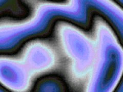
That's it. The other texture's formula cannot be deduced as easily, because I found it by trial and error. The formula looks like black magic, but it is simpler than it looks:
        sin (.03 (abs(x) + abs(y))) +
        sin (.03 (abs(x)^2 + abs(y)^2)) +
        sin (.03 (abs(x)^1.5 + abs(y)^1.5)) +
The result goes from -3 to 3, and must be scaled appropriately to change the range to 0..255 (you should already know how to do that from the plasma chapter).
How did I find that formula? abs(x)+abs(y) alone yields something similar to the first texture but gives a pattern of rhombs rather than circles (try to compute it for several points until you are convinced of that); putting it inside a sine avoids abrupt changes from black to white. The second term makes circles like in the first texture, but again the sine makes the shading more smooth. The last term gives rhombs with rounded edges (the exponent is half way from 1 to 2) and I added it only to make the thing more interesting.
Giving objects a trajectory
When you do effects that involve sprites, for example vectorballs or shadebobs (do you remember them?!?), you have to find a nice trajectory on which to place new objects. This is a perfect job for sines and cosines.
We'll derive the formula from the interference effect. I'll quote from that section of the article: "what the effect does is simply to shift the textures by a different amount on each frame"; in other words, what the cosines really give is the trajectory that is followed by the top-left corner of the texture -- the one at coordinates (0,0).
The formulas that we were using were
        x = cos (a t + c)
        y = cos (b t + d)
...and this will be perfect when a pretty simple trajectory is needed, for example for shadebobs. Here is a plot of a few functions of the form x = cos (a t), y = sin (b t), for values of a and c ranging from 3 to 6:
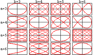
These curves are called the "Lissajous curves of order (a,b)". They correspond to a particular choice of the parameters c and d, that is c = d + PI/2. Also note that t can be a simple frame counter if you are using a cosine table (therefore the argument of the cosine will be from 0 to 255, or something like that), while if you use floating point math t will be incremented by a small quantity on every frame (like we did in the interference pseudocode).
Note that if a=b you get a circle... Of course it is not a coincidence, but to understand why I'll have to explain what sines and cosines actually mean.
Lissajous curves have many uses. They can be extended to three dimensions, like this:
        x = cos (a t) * cos(c t)
        y = cos (a t) * sin(d t)
        z = sin (b t)
If on your coding career you ever encounter "polar" and "spherical" coordinates -- you surely will -- come back here and compare the formulas for 2D and 3D Lissajous curves to those for polar and spherical coordinates, respectively. You'll find a striking similarity.
Also, you can use Lissajous curves whenever you need two values to change with some regularity, it does not matter if they are not x and y values: for example you can rotate a 3D model around two axes by PI cos(a t) and PI sin(b t) radians.
Never take this information for granted, however. Experiment a lot, try to imagine what trajectories come out when you square sines and cosines, take their absolute value, multiply a few of them, and so on; then check your guesses with a spreadsheet or a math program such as Matlab or Mathematica.
Shadebobs and wormies
Now, coding a shadebob will be a breeze. Here is an example:

This is part of a very simple intro that I wrote for the 13th birthday of my girlfriend's sister (the text means "Happy Birthday" in Italian, and the shadebob is a 13).
You have to write two bitmap drawing routines that, instead of coloring a pixel with the color indicated in the bitmap, add or subtract that color to the VRAM. Never draw the shadebob with light colors, because that would surely cause an overflow when you draw it many times with similar coordinates; in general, don't exceed a pixel value of 16.
Then, you have to ensure that only a certain number of copies of the shadebob are drawn at any time. To do so, the following pseudocode simply keeps an history of the last 64 places where the shadebob has been drawn:
    t = 0
    for every frame
        oldx = buffer[t & 63].x
        oldy = buffer[t & 63].y
        if t > 63 then
            subtract the shadebob at coordinates (oldx, oldy)

        newx = cos(a t)
        newy = sin(b t)
        buffer[t & 63].x = newx
        buffer[t & 63].y = newy
        add the shadebob at coordinates (newx, newy)
        t = t + 1
Here is the actual routine that I used in my intro. The change was needed to make the 13 readable, and is very simple: the latest position is overdrawn five times (to make the bob lighter) and made dimmer on the very next frame:
    t = 0
    for every frame
        if t >= 1 then
            subtract the shadebob at coordinates (newx, newy)
            subtract the shadebob at coordinates (newx, newy)
            subtract the shadebob at coordinates (newx, newy)
            subtract the shadebob at coordinates (newx, newy)

        oldx = buffer[t & 63].x
        oldy = buffer[t & 63].y
        if t > 63 then
            subtract the shadebob at coordinates (oldx, oldy)

        newx = cos(a t)
        newy = sin(b t)
        buffer[t & 63].x = newx
        buffer[t & 63].y = newy
        add the shadebob at coordinates (newx, newy)
        add the shadebob at coordinates (newx, newy)
        add the shadebob at coordinates (newx, newy)
        add the shadebob at coordinates (newx, newy)
        add the shadebob at coordinates (newx, newy)
        t = t + 1
Note that the balance between drawn and removed copies is preserved: on each frame, five copies of the shadebob are drawn and five are removed.
Wormies are very similar, but have more complex trajectories. Also, usually you redraw wormies from scratch on each frame because their components are opaque (the most recent ones overlap the older ones).
This one is taken from a 4k intro, "Never bored", by Ritz (see Hugi 21):
This one can easily become a complex effect, but there is very little math in it apart from sin/cos. As usual, you can get by with a little trial and error; here is a simple wormie:
        x = cos t + .7 * cos 3.02t
        y = sin t + .05 * sin 15.04t
My first step here was to take a circle and perturb it with a Lissajous curve of order (3,15). Then I also tweaked the order of the curve a bit to break its symmetry and make the wormie's behavior more interesting.
You can invent many variations on wormies like you can do with plasmas. For example, Ritz's wormie is three-dimensional and the balls that compose it are scaled so that the farthest are also the smallest. Also, the simplest possible wormie draws each ball for a fixed number of frames and then removes it, while Ritz makes the balls fade out slowly and also doesn't let them stay fixed at their original position, but moves them away as they get dimmer (I think).
Trigonometry? What's trigonometry?
Let's go back to Lissajous curves. I already pointed out that a curve of the form
        x = cos a t
        y = sin a t
is a circle, and that it is not a coincidence. In fact, by definition, if you have a circle of radius 1 and an angle x, (cos x, sin x) is the point on the circle whose radius makes an angle of x with the x axis:
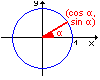
Angles are measured in a funny unit of measure that mathematicians love, called radian, with the property that 2PI radians equal exactly 360 degrees (a full tour around the circle).
Now we can describe any point on a circle of radius R by the angle a that it forms, by writing (x, y) as (R cos a, R sin a). These are called polar coordinates and will be useful for the next two effects, rotozooming and wormholes.
Rotozooming (also known as rototiling)
This effect is quite easily done and offers an easy way to test your understanding of basic "real" applications of sines and cosines (i.e. exploiting their definition and not treating them as simply nice curves). This screenshot is another section of my birthday intro:
Let's write a point in polar coordinates and rotate it by an angle da. It should be clear that the point's cartesian coordinates can be expressed as
        x = R cos (a)
        y = R sin (a)

        x' = R cos (a + da)
        y' = R sin (a + da)
respectively before and after rotation.
Now take for granted two trigonometric formulas that give the sine and cosine of the sum of two angles:
        cos (a + da) = cos(a) cos(da) - sin(a) sin(da)
        sin (a + da) = cos(a) sin(da) + sin(a) cos(da)
and plug it into the formulas for x' and y':
        x' = R cos(a) cos(da) - R sin(a) sin(da)
        y' = R cos(a) sin(da) + R sin(a) cos(da)
But is it worthwhile to map from cartesian to polar coordinates and back, twice for pixel? It looks like a good deal of work, and of course it is not necessary, because we can substitute the original x and y like this:
        x' = x cos(da) - y sin(da)
        y' = x sin(da) + y cos(da)
The beauty is that cos(da) and sin(da) are constant, and hence can be computed only once per frame!
For now, let's content of rotating every pixel in the bitmap without zooming. We could apply the equations that we have just found to obtain the screen (i.e. rotated) coordinates for each point of the bitmap, but this wouldn't do the tiling effect that is seen above and would not extend easily to zooming (you would plot many points to the same destination when each the image was made smaller, and leave holes when the image is enlarged).
Instead we want to proceed through all the pixels on screen and, one by one, find where it comes from on the texture image. There are two ways to find the required equation, i.e. brute force and reasoning. Brute force means solving the equations above for x and y rather than x' and y'; not so complicated, but if you think about it, you simply have to invert the rotation direction to reverse the transformation: if texture->screen is a clockwise rotation, screen->texture must be a counterclockwise rotation. So the equations are simply:
        x = x' cos(da) - y' sin(da)
        y = x' sin(da) + y' cos(da)
And here is the pseudocode. Why I am using a table to store sines and cosines will be clear later. Also note that I am not doing the four multiplications on every pixel, and that you must compensate so that the rotation is around the center of the screen rather than around the top-left corner:
     enter gfx mode and set the palette
     for i := 0 to 255 do
       cosTable[i] := cos (i * 2*PI/256)
       sinTable[i] := sin (i * 2*PI/256)
     end;

     angle := 0
     for each frame
       cosine := cosTable[angle]
       sine := sinTable[angle]

       for sy := 0 to maxy - 1 do
         tx := (-maxx / 2) * cosine - (-maxy / 2) * sine
         ty := (-maxx / 2) * sine + (-maxy / 2) * cosine
         for sx := 0 to maxx - 1 do
           color := texture[tx][ty];
           plot (sx,sy) with this color
           tx := tx + cosine
           ty := ty + sine
         end;
       end;
     end;
Now we want to add zooming as well. The equations for zooming are simply
        x' = k x
        y' = k y
with k>1 giving enlarged images and k<1 giving smaller images. These are easily inverted to x = x'/k, y = y'/k to transform screen coordinates to texture coordinates. We can also combine them with the equations for rotations:
        x = x' cos(da) / k - y' sin(da) / k
        y = x' sin(da) / k + y' cos(da) / k
Now, what we will use to vary k over time? Of course a cosine curve! For example, if you want the curve to oscillate between 50% and 250% of its original size, just put k = 1.5+sin(a t).
You still have only two coefficients in the equations: only, instead of cos(da) and sin(da), they are cos(da)/k and sin(da)/k. Turning "rototiling" into "rotozooming" is then surprisingly simple: you just have to tweak the cosine and sine table:
     for i := 0 to 255 do
       cosTable[i] := cos (i * 2*PI/256) * (1.5 + sin (i * 2*PI/256))
       sinTable[i] := sin (i * 2*PI/256) * (1.5 + sin (i * 2*PI/256))
     end;
That's it!
Starfields, or the basics of 3D projection
This effect does not have a single sine or cosine in it :-) but it is propedeutic to another one, wormholes, which has a lot of them! Starfields are yet another of those effects that everybody codes once in his life, because they are the simplest three-dimensional effect one could imagine.
A star field should give the idea of moving at (ridiculously) high speed in space, seeing stars coming towards you as you miraculously dodge all of them.
A basic starfield is very simple: you have a set of 3D points to be plotted on the screen, and the movement effect is achieved by simply decreasing the z coordinate (this shoule make sense after the paragraph on rotozooming: the imaginary spaceship moves towards increasing z coordinates, so the stars "see" the inverse transformation which is to decrease z's). and redisplaying the results. The formula for 3D to 2D projection (read: conversion) is:
     xs = d * x / z
     ys = d * y / z
This should make perfect sense. As the object moves away from you (increasing z coordinates), the screen coordinates (xs,ys) tend to (0,0). The dparameter is simply used to scale the coordinates so that the objects occupy a meaningful fraction of the screen and can be set for example to 256 or another power of two.
First of all you create a set of random stars with a fixed z and random (x,y). On each frame you decrement the z coordinates, compute the screen coordinates and, if they got out of the screen, you replace the star with a newly created one. Since far objects are also very dim, the color is usually given based on the z coordinate, with a shade going from black to light violet, or something like that.
Starfields have many variations that can make them more interesting. You can make the rendering more realistic by drawing the stars as short lines (possibly antialiased...) which give the impression of the persistence of images on the human eye; you can tilt the viewpoint so that it looks like the spaceship is really dodging the stars; you can draw the stars in different sizes depending on how near they are. To do so, you need a very basic knowledge of 3D math: on one hand, I don't have the space and the intention to treat all this here; on the other hand, actually you might be able to deduce it from what I said on 2D rotation, and anyway there are plenty of tutorials that cover that. Creating all these variations will be a great way to practice with basic 3D math.
Wormholes
The wormhole effect is a good way to end this tutorial, because it combines many of the aspects that I have covered: trajectories, 3D, and basic trigonometry. A wormhole can be seen in 2nd reality, by the Future Crew (nothing less):
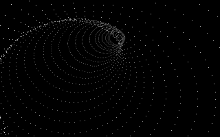
To draw a wormhole, you simply have to draw many circles at different z coordinates. The perception of depth can be improved by giving darker colors for bigger z's.
The centers of the circles move on a Lissajous curve. You need to store the center coordinates for a certain number of circles, and draw them on each frame with a different z: on each frame, the z will get smaller because the circles will move towards the viewer (whose z is 0).
Now let's go down to the details. How do we draw a 3D circle? In fact it is pretty easy, because the points on the circle will have a constant z (the circle directly faces the viewer). So if the center is (x0, y0, z0) and the radius is r, the points on the circle are (x0 + r cos a, y0 + r sin a, z0). To do perspective projection, you simply have to scale appropriately x0, y0, and the radius as well.
The pseudocode for the drawcircle function is then
    drawcircle (x0, y0, z0, r, color):
      xc := d * x0 / z0
      yc := d * y0 / z0
      rc := d * r / z0

      for t := 0 to 63 do
        x = xc + rc * cos(t * 2*PI/64)
        y = yc + rc * sin(t * 2*PI/64)
        if (x,y) is on screen, plot it with the given color
      end;
Of course you'd better have a sine/cosine table. Now, let's go with the whole effect, using 64 circles.
     enter gfx mode and set the palette
     t := 0
     for each frame
       x0[t & 63] := cos (3*t * 2*PI/256) + 1
       y0[t & 63] := sin (5*t * 2*PI/256) + 1

       z = 200
       for i = t - 63 to t do
         if i > 0 then
           drawcircle (x0[i & 63], y0[i & 63], z, 1, color)
           z = z + 5
         end;
       end;
       t := t + 1
     end;
To understand how 3D projection works, adjust the initial value of z (200) and the value of d (not given in the source above). You should notice that smaller z's must be compensated with smaller d's, but the compensation will not be exact, because picking small values of z will distort the image like if you were using a wide-angle or fisheye lens on a camera.
If you feel brave, you can get a tutorial on drawing filled polygons and turn this wormhole into a solid one. Just compute pairs of points on two adjacent circles and draw filled quadrilaterals.
Or, learn something on 3D rotation and try to do a real 3D wormhole. That is, the trajectory will not be given directly by a Lissajous curve, but the curve will only give the angle between the z axis and the direction that the wormhole assumes (you need spherical coordinates to do that); the circles then will be tilted so that they are always perpendicular to the direction, and as you move in the wormhole the viewer will also tilt to align with the direction.
This is quite complex, so here are a couple of hints. First, you can easily compute the coordinates a circle and the direction assumed by the wormhole: store in an array both the direction of the z axis (0,0,1) and the coordinates of the points on a circle perpendicular to the z axis (r cos t, r sin t, 0); then, rotate all these points by the same angles, and magically the points on the circle will stay perpendicular to the axis.
Second, remember that angles are always relative to the position of the viewer. For example, now I'm facing the monitor of my PC (0 degrees), but if I turn my head to the left (+90 degrees), the monitor will be on my right (-90 degrees). In other words, if an object makes an angle a with the z axis, and the viewer makes an angle b with the z axis, you must rotate the object by an angle of a-b.
The reason for the - sign is similar to what we did when rotozooming: there, if we applied a transformation on the texture, we would have applied the inverse transformation to the screen coordinates; similarly, if we apply a transformation on the viewer, we must apply the opposite transformation to the objects.
What's next?
Well, the effects in this articles should give you enough material to experiment with and to receive some satisfaction from your first productions. Remember that ultimate 3D can be a goal, but it takes time, and starting with simple things will be easier and more interesting as well. People will appreciate demos with these simple effects because demos are not judged only for their technical quality, but also for their design and for their purpose.
Take a look at productions which you know to have few or no 3D scenes (there is no preferred category -- as outstanding examples of this, consider the 4k Mesha or the Ibiza demo), and try to look at them from a mathematical point of view. Of course, do this after having enjoyed the spectacle! Try to recreate what you see or some variation on it. If it looks too complex, don't worry, try something else. If you care, try some of the "exercises" that I propose, and when you feel ready, go for some 3D as well. The really important things are that you experiment a lot, and that you enjoy yourself!
--
|_  _  _ __
|_)(_)| ) ,'
-------- '-._